Science requires reproducibility, not only to ensure that your results are generalizable but also to make your life easier. One overlooked aspect of of learning data science is creating consistent and clear organization of your projects and learning how to keep your data safe and easily searchable.
Quick note (TODO)
Citations incoming. Please note that much of this document does not contain original material. References are listed at the end of the chapter (I still need to get my .bib files in order to give proper attribution).
Why care about data management?
Computing is now an essential part of research. This is outlined beautifully in the paper, “All biology is computational biology” by Florian Markowetz. Data is getting bigger and bigger and we need to be equipped with the tools for storing, manipulating, and communicating insights derived from it. However, most researchers are never taught good computational practices. Computational best practices are imperitive. Implementing best (or good enough) practices can improve reproducibility, ensure correctness, and increase efficiency.
File Management
File types and file names
As a data scientist you’ll be dealing with a lot of files but have you ever considered what a file is? Files come in all shapes and formats. Some are very application specific and require specialized programs to open. For example, consider DICOM files that are used to store and manipulate radiology data. Luckily, in bioinformatics we tend to deal mainly with simple, plain text files, most often. Plain text files are typically designed to be both human and machine-readable. If you have the choice of saving any data, you should know that some formats will make your life easier. Certain file formats like TXT, CSV, TSV, JSON, and YAML are standard plain text file formats that are easy to share and easy to open and manipulate. Because of this, you should prefer to store your data in machine-readable formats. Avoid .xlsx files for storing data. Prefer TXT, CSV, TSV, JSON, YAML, and HDF5.
If you have very large text files then you can use compression utilities to save space. Most bioinformatics software is designed to work well with gzip compressed data. gzip is a relatively old compression format. You could also consider using xz as a means to compress your data - just know that xz compression is less supported across tools.
File naming
File naming is important but often overlooked. You want your files to be named logically and communicate their contents. You also want your files to be named in a way that a computer can easily read. For example, spaces in filenames are a royal pain when manipulating files on the command line.
To ensure filenames are computer friendly, don’t use spaces in filenames. Use only letters, numbers, and “-” “_” and “.” as delimiters. For example:
# Baddata for jozef.txt# Okaydata-for-jozef.txt# Best2023-11-09_repetitive-element-counts.txt
Quiz
I have a directory with the following files:
a.txtb.txtc.txtfile with spaces in the name.txtsome other file.txt
What does the following code return? (Expected: For each file in the directory print the filename)
A simple alternative here is to use a text document with the basenames the files you want to loop over and then loop over the lines of the file instead.
It cannot be stressed enough how important filenames can be for an analysis. To get the most out of your files and to avoid catastrpohic failures, you should stick to some basic principles for naming files. First, use consistent and unique identifiers across all files that you generate for an experiment. For example, if you’re conducting a study that has both RNA-seq and ATAC-seq data performed on the same subjects, don’t name the files from the RNA-seq experiment subject1.fq.fz and the files from the ATAC-seq experiment control_subject1.fq.gz if they refer to the same sample. For small projects, it’s fairly easy to create consistent and unique IDs for each subject. For large projects unique random IDs can be used.
For example, the following filenames would be bad:
These are better. Why are they better? They are consistent. The delimiter is consistent between the words (“_“) and each of the words represents something meaningful about the sample. These filenames also do not contain any spaces and can easily be parsed automatically.
File naming best practices also apply to naming executable scripts. The name of the file should describe the function of the script. For example,
01_align_with_STAR.sh
is better than simply naming the file
01_script.sh
Pro-tip
One easy way to create unique random IDs for a large project is to concatenate descriptions and take the SHA/MDA5 hashsum.
The term tidy data was defined by Hadley Wickham to describe data which is amenable to downstream analysis. Most people are familiar with performing a quick and dirty data analysis in a program like Excel. You may have also used some of Excel’s fancy features for coloring cells, adding bold and underlines to text, and formatting cells with other decorations. All of this tends to just be extra fluff. If you format you data properly then it will be much easier to perform downstream analysis on and will not require the use of extra decorations. This is true even in Excel!
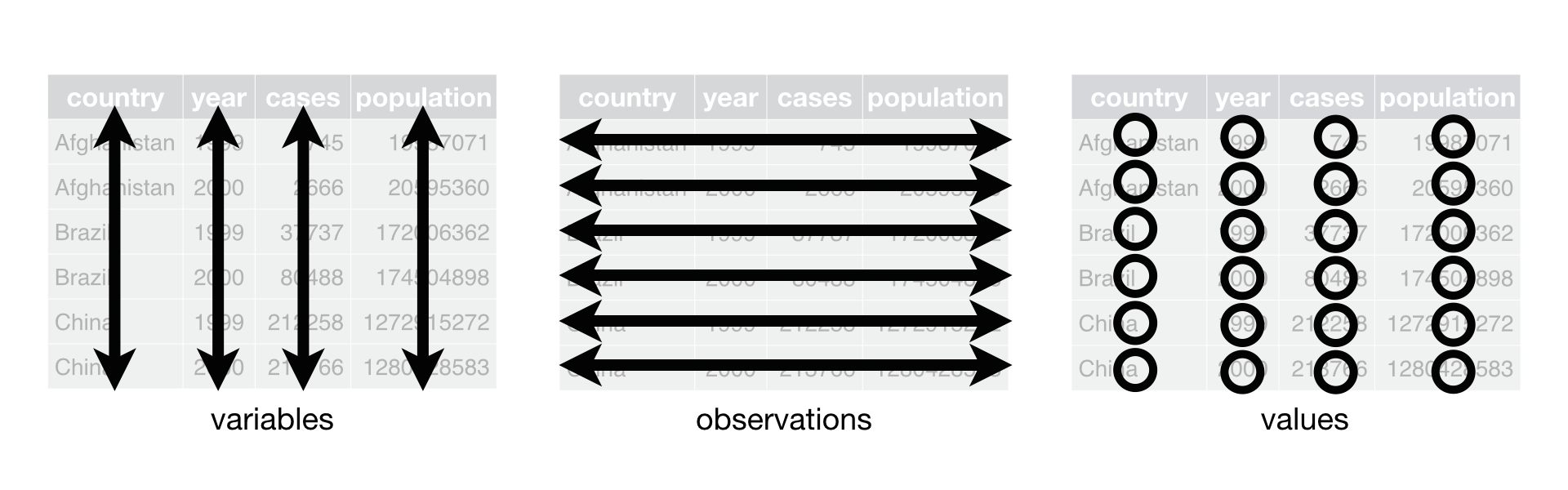
To conform to the requirements of being tidy, the data should follow some simple principles:
Each variable must have its own column.
Each observation must have its own row.
Each value must have its own cell.
Don’t cram two variables into one value. e.g. “male_treated”.
Don’t embed units into data. e.g. “3.4kg”. Instead, put in column name e.g. “weight_kg” = 3.4
Once your data is in this format, it can easily be read into downstream programs like R, or parsed with command line text editing programs like sed.
The iris dataset in R provides a classic example of this format
see R arrow for more details. There’s also the nanoparquet package which provides a light weight reader/writer for parquet files.
Untidy(?) data
Some data formats are not amenable to the ‘tidy’ structure, i.e. they’re just not best represented as long tables. For example, large/sparse matrices, geo-spatial data, R objects, etc.the lesson here is to store data in the format that is most appropriate for the data. For example, don’t convert a matrix to a long format and save as a tsv file! Save it as an .rds file instead. Large matrices can also be efficiently stored as HDF5 files. Sparse matrices can be saved and accessed eficiently using the Matrix package in R. And if you are accessing the same data often, consider storing as a SQLite database and accessing with dbplyr or sqlalchemy in Python. The main point is don’t force data into a format that you’re familiar with only because you’re familiar with that format. This will often lead to large file sizes and inefficient performance.
Save and lock all raw data
Keep raw data in its unedited form. This includes not making changes to filenames. In bioinformatics, it’s common to get data from a sequencing facility with incomprehensible filenames. Don’t fall victim to the temptation of changing these filenames! Instead, it’s much better to keep the filenames exactly how they were sent to you and simply create a spreadsheet that maps the files to their metadata. In the case of a sample mix-up, it’s much easier to make a change to a row in a spreadsheet then to track down all of the filenames that you changed and ensure they’re correctly modified.
Once you have your raw data, you don’t want the raw data to change in any way that is not documented by code. To ensure this, you can consider changing file permissions to make the file immutable (unchangable). Using bash, you can change file permissions with:
chattr +i myfile.txt
If you’re using Excel for data analysis, lock the spreadsheet with the raw data and only make references to this sheet when performing calculations.
Large files
You’ll probably be dealing with files on the order of 10s of GBs. You do not want to be copying these files from one place to another. This increases confusion and runs the risk of introducing errors. Instead avoid making copies of large local files or persistent databases and simply link to the files.
You can use use soft links. A powerful way of finding an linking files can be done with find
# Link all fastq files to a local directoryfind /path/to/fq/files -name"*.fq.gz")-exec ln -s {} . \;
If using R, you can also sometimes specify a URL in place of a file path for certain functions.
# Avoid downloading a large GTF file - reads GTF directly into memoryurl <-"https://ftp.ebi.ac.uk/pub/databases/gencode/Gencode_human/release_44/gencode.v44.annotation.gtf.gz"gtf <- rtracklayer::import(url)
Backups
There are two types of people, those who do backups and those who will do backups.
The following are NOT backup solutions:
Copies of data on the same disk
Dropbox/Google Drive
RAID arrays
All of these solutions mirror the data. Corruption or ransomware will propagate. For example, if you corrupt a file on your local computer and then push that change to DropBox then the file on DropBox is now also corrupted. I’m sure some of these cloud providers have version controlled files but it’s better to just avoid the problem entirely by keeping good backups.
Use the 3-2-1 rule:
Keep 3 copies of any important file: 1 primary and 2 backups.
Keep the files on 2 different media types to protect against different types of hazards.
Store 1 copy offsite (e.g., outside your home or business facility).
A backup is only a backup if you can restore the files!
Project Organization
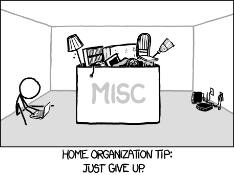
Look familiar?
Project structure
One of the most useful changes that you can make to your workflow is the create a consistent folder structure for all of your analyses and stick with it. Coming up with a consistent and generalizable structure can be challenging at first but some general guidelines are presented here and here
First of all, when beginning a new project, you should have some way of naming your projects. One good way of naming projects is to each project a descriptive name and append the date the project was started. For example, brca_rnaseq_2023-11-09/ is better than rnaseq_data/. In six months when a collaborator wants their old BRCA data re-analyzed you’ll thank yourself for timestamping the project folder and giving it a descriptive name.
My personal structure for every project looks like:
Prefixing the project directory with the ISO date allows for easy sorting by date
a README text file is present at the top level of the directory with a short description about the project and any notes or updates
data/ should contain soft links to any raw data or the results of downloading data from an external source
doc/ contains metadata documents about the samples or other metadata information about the experiment
results/ contains only data generated within the project. It has sub-directories for figures/, data-files/ and rds-files/. If you have a longer or more complicated analysis then add sub-directories indicating which script generated the results.
scripts/ contains all analysis scripts numbered in their order of execution. Synchronize the script names with the results they produce.
If using Rstudio, include an .Rproj file at the top level of your directory. Doing this enables you to use the here package to reference data within your project in a relative fashion. For example, you can more easily save data with:
Always document all steps you used to generate the data that’s present in your projects. This can be as simple as a README with some comments and a wget command or as complex as a snakemake workflow. The point is, be sure you can track down the exact source of every file that you created or downloaded.
For example, a README documenting the creation of the files needed to generate a reference index might look like:
For more complicated steps include a script. e.g. creating a new genome index, subsetting BAM files, accessing data from NCBI, etc.
Pro-tip
A simple way to build a data pipeline that is surprisingly robust is just to create scripts for each step and number them in the order that they should be executed.
01_download.sh02_process.py03_makeFigures.R
You can also include a runner script that will execute all of the above. Or, for more consistent workflows, use a workflow manager like Nextflow, Snakemake, WDL, or good ole’ GNU Make
Manual version control
Version control refers to the practice of tracking changes in files and data over their lifetime. You should always track any changes made to your project over the entire life of the project. This can be done either manually or using a dedicated version control system. If doing this manually, add a file called “CHANGELOG.md” in your docs/ directory and add detailed notes in reverse chronological order.
For example:
## 2016-04-08

* Switched to cubic interpolation as default.
* Moved question about family's TB history to end of questionnaire.

## 2016-04-06

* Added option for cubic interpolation.
* Removed question about staph exposure (can be inferred from blood test results).
If you make a significant change to the project, copy the whole directory, date it, and store it such that it will no longer be modified. Copies of these old projects can be compressed and saved with tar + xz compression
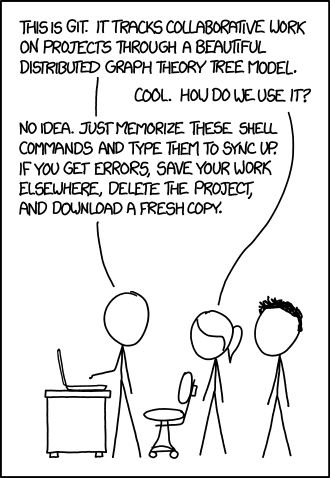
git is probably the de facto version control system in use today for tracking changes across software projects. You should strive to learn and use git to track your projects. Version control systems allow you to track all changes, comment on why changes were made, create parallel branches, and merge existing ones.
git is primarily used for source code files. Microsoft Office files and PDFs can be stored with Github but it’s hard to track changes. Rely on Microsoft’s “Track Changes” instead and save frequently.
It’s not necessary to version control raw data (back it up!) since it shouldn’t change. Likewise, backup intermediate data and version control the scripts that made it.
Be careful committing sensitive information to GitHub
Software
Quick tips to improve your scripts
Place a description at the top of every script
The description should indicate who the author is. When the code was created. A short description of what the expected inputs and outputs are along with how to use the code. You three months from now will appreciate it when you need to revisit your analysis
For example:
#!/usr/bin/env python3# Gennaro Calendo# 2023-11-09# # This scripts performs background correction of all images in the # user supplied directory## Usage ./correct-bg.py --input images/ --out_dir out_directory#from image_correction import background_correctfor img in images: img = background_correct(img) save_image(img, "out_directory/corrected.png")
Decompose programs into functions
Functions make it easier to reason about your code, spot errors, and make changes. This also follows the Don’t Repeat Yourself principle aimed at reducing repetition by replacing it with abstractions that are more stable
Compare this chunk of code that rescales values using a min-max function (0-1)
Which is easier to read? Which is easier to debug? Which is more efficient?
Give functions and variables meaningful names
Programs are written for people and then computers
Use variable and function names that are meaningful and correct
Keep names consistent. Use either snake_case or camelCase but try not to mix both
Bad:
lol <-1:100mydata <-data.frame(x =c("Jozef", "Gennaro", "Matt", "Morgan", "Anthony"))f <-function(x, y, ...) {plot(x = x, y = y, main ="Scatter plot of x and y", ...)}
Better:
ages <-1:100bioinfo_names <-data.frame(Name =c("Jozef", "Gennaro", "Matt", "Morgan", "Anthony"))plotScatterPlot <-function(x, y, ...) {plot(x = x, y = y, main ="Scatter plot of x and y", ...)}
Do not control program flow with comments
this is error prone and makes it difficult or impossible to automate
Use if/else statements instead
Bad:
# Download the file#filename <- "data.tsv"#url <- "http:://example.com/data.tsv"#download.file(url, filename)# Read in to a data.framedf <-read.delim("data.tsv", sep="\t")
Pick a style guide and stick with it. If using R, the styler package can automatically clean up poorly formatted code. If using Python, black is a highly opinionated formatter that is pretty popular. Although, I think ruff is currently all the rage with the Pythonistas these days.
This is R specific. I’ve seen this pop up with folks who are strong tidyverse adherents. I get it, that’s the direction of the piping operator. However, this right-hand assignment flies in the face of basically every other programming language, and since code is primarily read rather than executed, it’s much harder to scan a codebase and understand the variable assignment when the assignments can be anywhere in the pipe!
Don’t do this
data |>select(...) |>filter(...) |>group_by(...) |>summarize(...) -> by_group
It’s much easier to look down a script and see that by_group is created by all of the piped operations when assigned normally.
by_group <- data |>select(...) |>filter(...) |>group_by(...) |>summarize(...)
Summary
Data management
Save all raw data and don’t modify it
Keep good backups and make sure they work. 3-2-1 rule
Use consistent, meaningful filenames that make sense to computers and reflect their content or function
Create analysis friendly data
Work with/ save data in the format that it is best suited to
Project Organization
Use a consistent, well-defined project structure across all projects
Give each project a consistent and meaningful name
Use the structure of the project to organize where files go
Tracking Changes
Keep changes small and save changes frequently
If manually tracking changes do so in a logical location in a plain text document
Use a version control system
Software
Write a short description at the top of every script about what the script does and how to use it
Decompose programs into functions. Don’t Repeat Yourself
Give functions and variables meaningful names
Use statements for control flow instead of comments
Use a consistent style of coding. Use a code styler